Chapter 3 Writing Tutorial Content

Now that you have your environment set up, let’s learn how to create compelling tutorial content using R Markdown. This chapter covers the essential techniques for writing effective GitBook tutorials.

3.1 Project Structure with .Rmd Files

Each .Rmd file in your project becomes a chapter in your GitBook. The structure is simple:

my-tutorial/
|-- index.Rmd          # Main page (Chapter 0)
|-- 01-chapter1.Rmd    # Chapter 1
|-- 02-chapter2.Rmd    # Chapter 2
|-- 03-chapter3.Rmd    # Chapter 3
`-- ...

3.1.1 File Naming Convention

• index.Rmd: Always the main/first page
• 01-intro.Rmd: Use numbers for ordering
• XY-descriptive-names.Rmd: Use descriptive names after numbers

3.2 Headings Create Sections

Headings automatically create your table of contents and navigation structure:

# Chapter Title {#chapter-id}

## Main Section

### Subsection  

#### Sub-subsection

3.2.1 Important Notes:

• # Chapter Title creates a new chapter
• {#chapter-id} creates an ID for cross-referencing
• Only use # for chapter titles in chapter files
• Use ##, ###, #### for sections within chapters

3.3 Code Chunks: The Heart of R Tutorials

Code chunks are what make R Markdown special. They execute R code and display the results:

3.3.1 Basic Code Chunk

```{r}
# This is R code
x <- c(1, 2, 3, 4, 5)
mean(x)
```

## [1] 3

3.3.2 Code Chunk Options

Control how your code appears and executes:

```{r your-chunk-name, echo=TRUE, eval=TRUE, fig.cap="Simple Line Plot"}
# echo=TRUE: Show the code
# eval=TRUE: Run the code  
# fig.cap: Caption for figures
plot(1:10, 1:10)
```

Here’s the actual chunk in action:

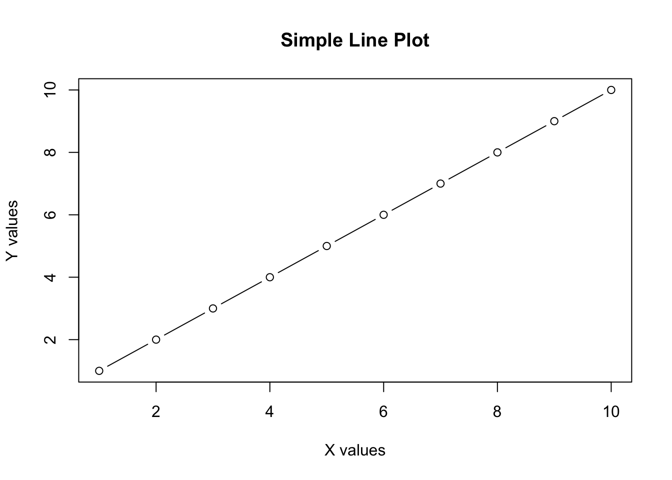
Figure 3.1: Simple Line Plot

Common options:

• echo=FALSE: Hide code, show output
• eval=FALSE: Show code, don’t run it
• include=FALSE: Run code, don’t show anything
• message=FALSE: Hide messages
• warning=FALSE: Hide warnings

3.4 Creating Plots and Visualizations

R excels at creating beautiful plots:

library(ggplot2)
data(mtcars)

ggplot(mtcars, aes(x = mpg, y = hp)) +
  geom_point(aes(color = factor(cyl))) +
  labs(title = "Horsepower vs MPG",
       x = "Miles per Gallon",
       y = "Horsepower",
       color = "Cylinders") +
  theme_minimal()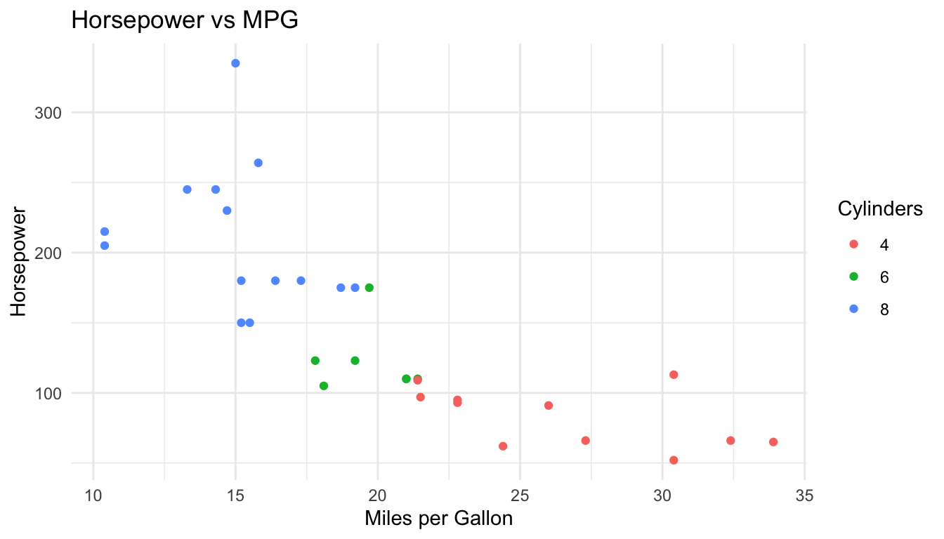

Figure 3.2: Sample Scatter Plot

3.5 Inline R Code

You can embed R results directly in your text using inline code:

The mean of mtcars$mpg is r round(mean(mtcars$mpg), 2) miles per gallon.

The mean of mtcars$mpg is 20.09 miles per gallon.

3.6 Mathematical Notation

LaTeX syntax works beautifully in GitBooks:

3.6.1 Inline Math

The formula is $y = mx + b$ where $m$ is the slope.

Result: The formula is \(y = mx + b\) where \(m\) is the slope.

3.6.2 Block Math

$$
\bar{x} = \frac{1}{n} \sum_{i=1}^{n} x_i
$$

Result: \[ \bar{x} = \frac{1}{n} \sum_{i=1}^{n} x_i \]

3.7 Cross-References and Links

3.7.1 Referencing Figures and Tables

See Figure \@ref(fig:plot-example) for the scatter plot.

Result: See Figure 3.2 for the scatter plot.

3.7.2 Referencing Sections

As we learned in Chapter \@ref(intro), GitBook format is powerful.

Result: As we learned in Chapter 1, GitBook format is powerful.

3.7.3 Creating Tables

knitr::kable(
  head(mtcars[, 1:4]), 
  caption = "First few rows of mtcars dataset",
  booktabs = TRUE
)

Table 3.1: First few rows of mtcars dataset

	mpg	cyl	disp	hp
Mazda RX4	21.0	6	160	110
Mazda RX4 Wag	21.0	6	160	110
Datsun 710	22.8	4	108	93
Hornet 4 Drive	21.4	6	258	110
Hornet Sportabout	18.7	8	360	175
Valiant	18.1	6	225	105

Reference it with: Table \@ref(tab:cars-table)

3.8 Optional Enhancements

3.8.1 Footnotes

Add footnotes for additional information. First, reference the footnote, then define what the footnote reads. Footnotes will be placed at the bottom of the page automatically.

This is the text where the footnote is referenced[^note1].
[^note1]: This is the content of the footnote.

Result:

This is the text where the footnote is referenced¹.

(Scroll to the bottom of the page to see the footnote.)

3.8.2 Citations with BibTeX

First, create a references.bib file:

@book{wickham2016r,
  title={R for data science: import, tidy, transform, visualize, and model data},
  author={Wickham, Hadley and Grolemund, Garrett},
  year={2016},
  publisher={O'Reilly Media}
}

Then cite it:

According to @wickham2016r, data science is a powerful approach.

3.8.3 Adding Images

![Caption for image](path/to/image.png)

Or with more control:

```{r, fig.cap="My Image", out.width="50%", eval=FALSE}
knitr::include_graphics("path/to/image.png")
```

3.8.4 Callouts and Special Blocks

Create attention-grabbing callouts:

> **Note:** This is an important note that readers should pay attention to.

> **Warning:** Be careful with this command as it might delete files.

> **Tip:** Here's a helpful tip to make your work easier.

Results:

Note: This is an important note that readers should pay attention to.

Warning: Be careful with this command as it might delete files.

Tip: Here’s a helpful tip to make your work easier.

---

1. And this is the content of the footnote.↩︎